Black Hole Optics 8.7

A software tool for simulating optical imaging in general curved spacetime, designed for scientists and practitioners working in astrophysics and theoretical physics. It provides a means for the detailed study of optical phenomena in gravitationally curved spacetime, including the analysis of light ray trajectories and their curvature around massive objects such as black holes. You can perform optical imaging simulations based on user-defined spacetime metrics, allowing you to explore different theoretical scenarios and models in relation to general relativity. It offers numerical methods and computational techniques to analyze properties of black holes, including event horizons, singularities, and curvature of spacetime. Explore the dynamics of optical phenomena in the vicinity of black holes with the ability to generate animations of the observer's motion along geodesic trajectories and follow their evolution at different points in time. Gain a useful tool for creating and testing theoretical models and hypotheses in astrophysics.

In the first video, the geodesics went against the direction of rotation of the black hole. In the second video of the black hole is simulated going around a highly inclined near-polar orbit, so that the optics of the rings can be seen. Here it is worth noting the brightening where the direction of the ring's orbit goes against the observer. Because the orbital velocity is relativistic, the brightening and color shift is significant.

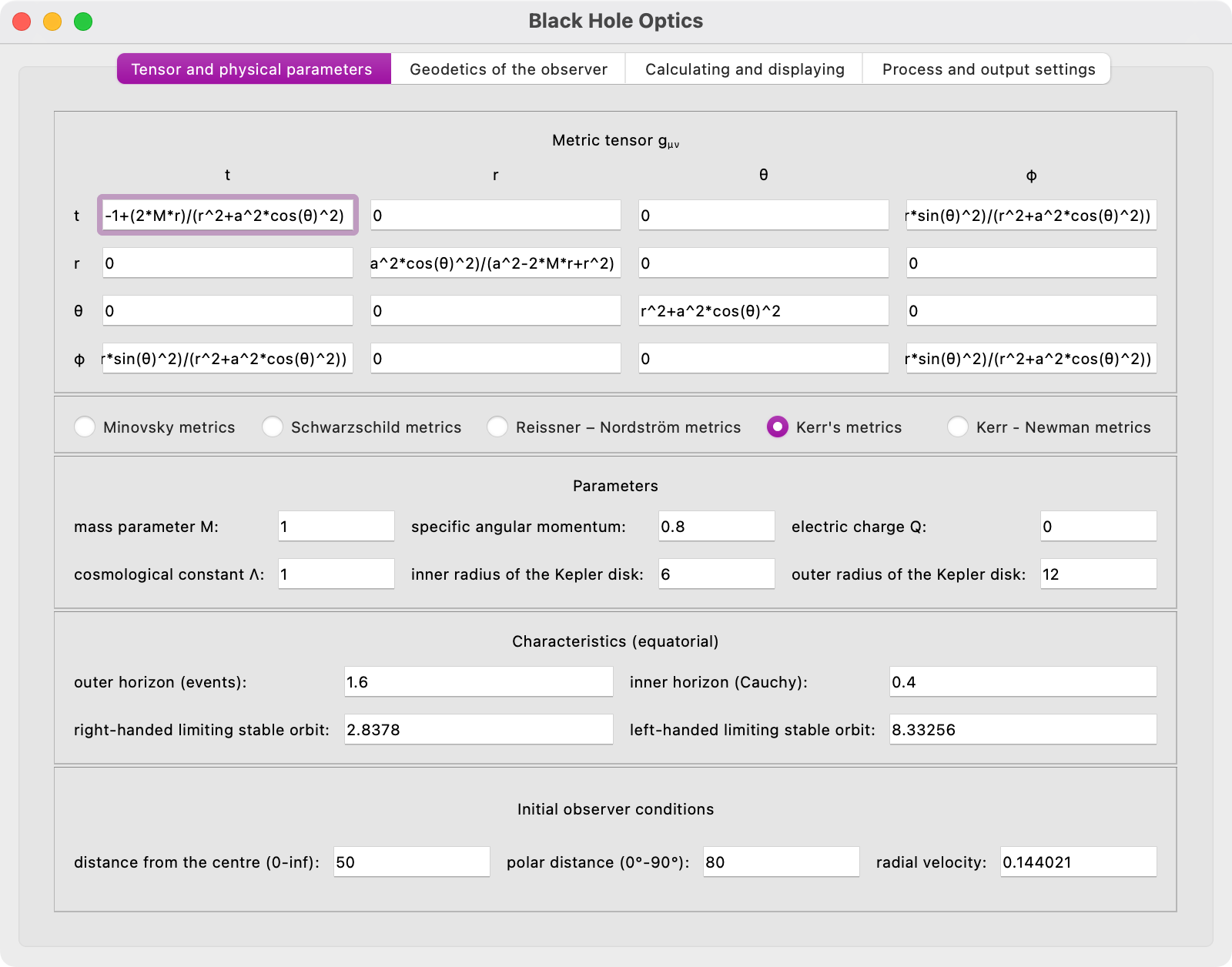
You can specify the tensor manually, but be sure to follow the syntax as you see it in the default metrics. You must type * when multiply. You must not put spaces between characters. If the program crashes, try writing the formula in a different form. So far, I've concentrated entirely on the calculations. The program is not yet tuned to resist input errors.

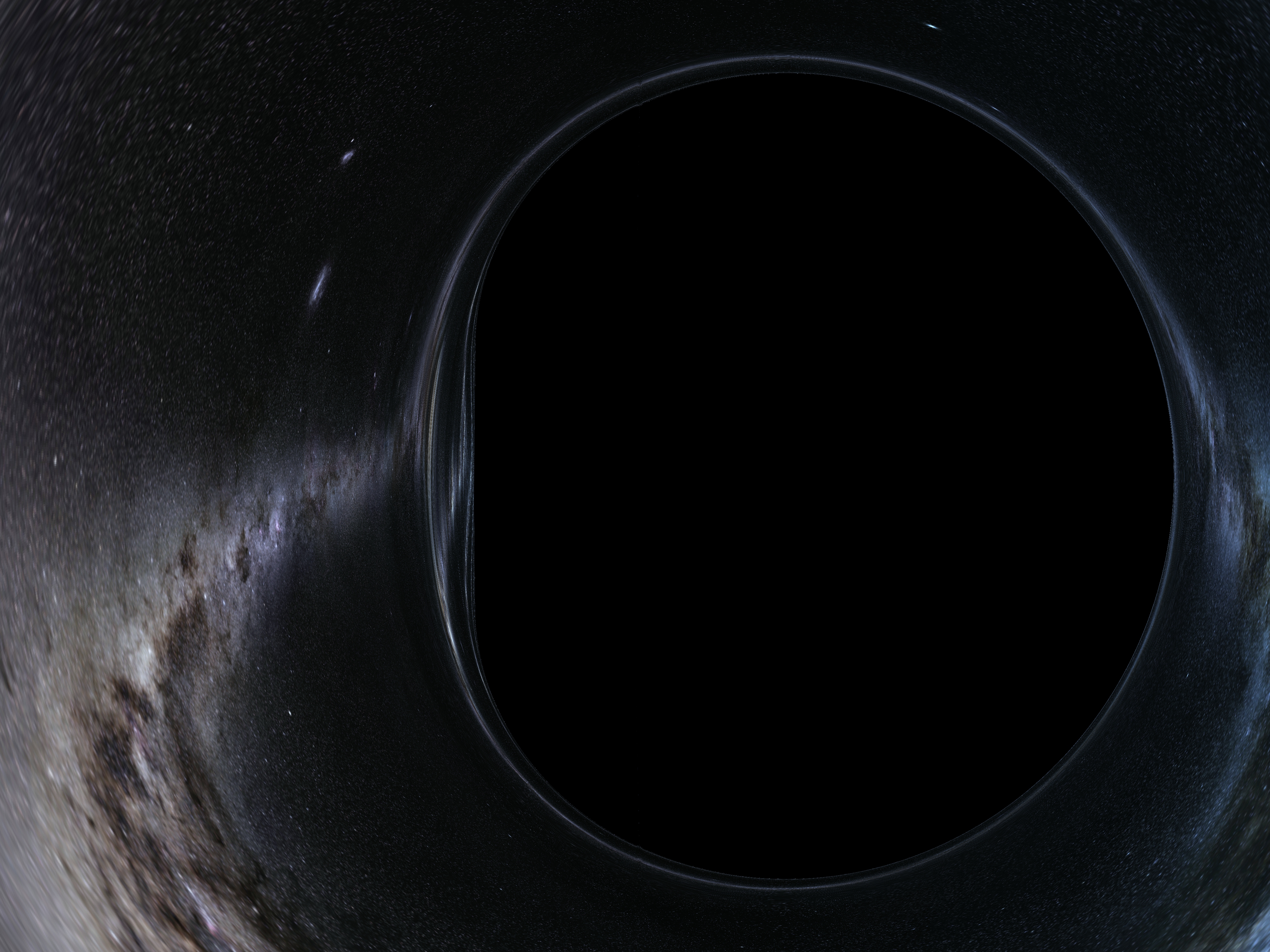
If you don't load the background image (which can be any size, but preferably 2:1 with distortion at the poles for a correct 360° view), you will see a green checkerboard. Its color will also be subject to redshift.

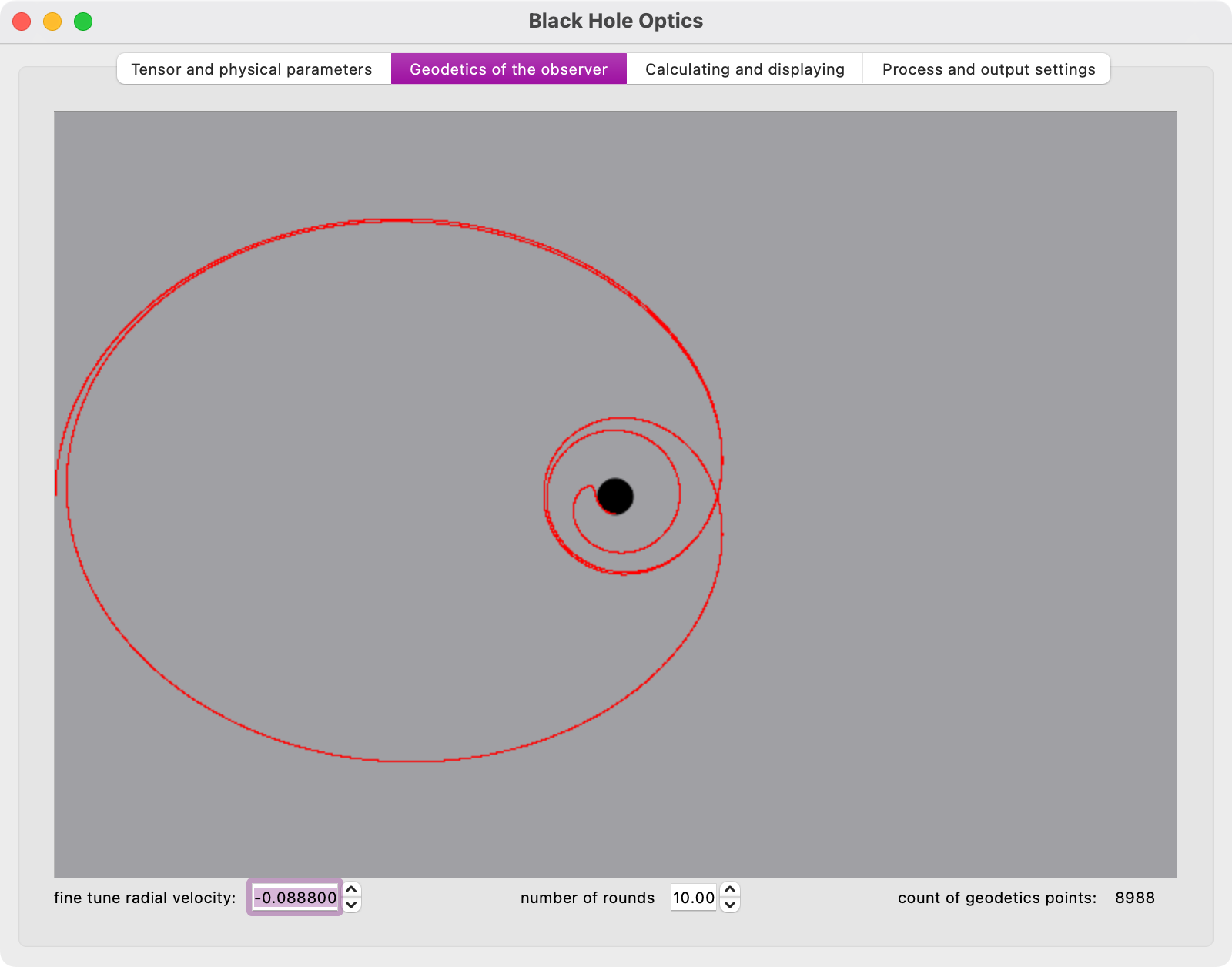
You can specify its distance from the origin, its polar distance and its velocity magnitude. The direction of the velocity vector is rigidly defined as parallel to the equatorial plane and perpendicular to the line joining the observer and the centre of the coordinates. Thus, an arbitrary direction cannot be specified, but by defining the entire orbit, an arbitrary direction can be achieved over the course of the orbit. Once the radial and polar distances have been entered, the velocity corresponding to the spherical motion is calculated for this, which can then be edited, but preferably on next tab specifically designed for this purpose.

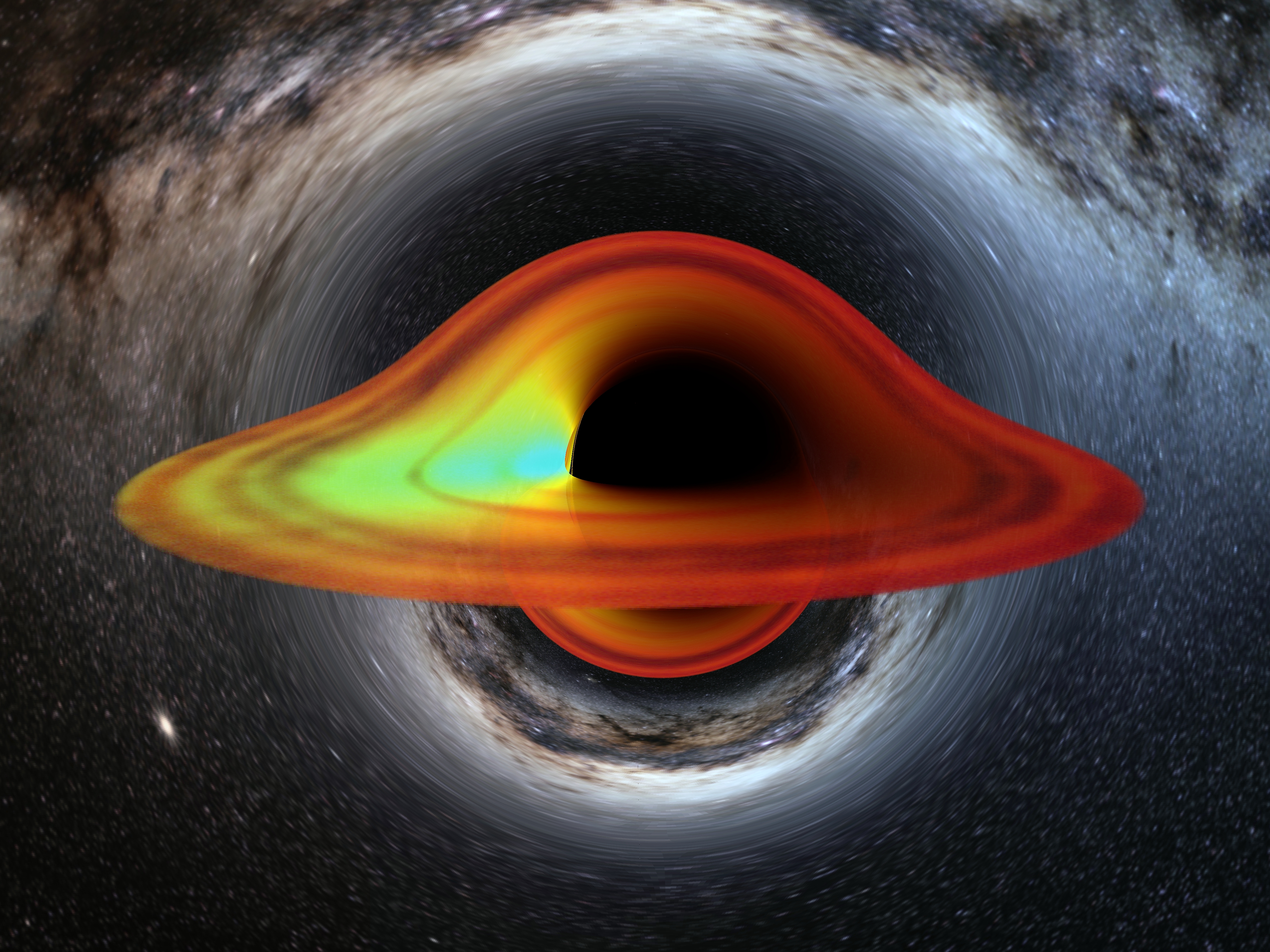
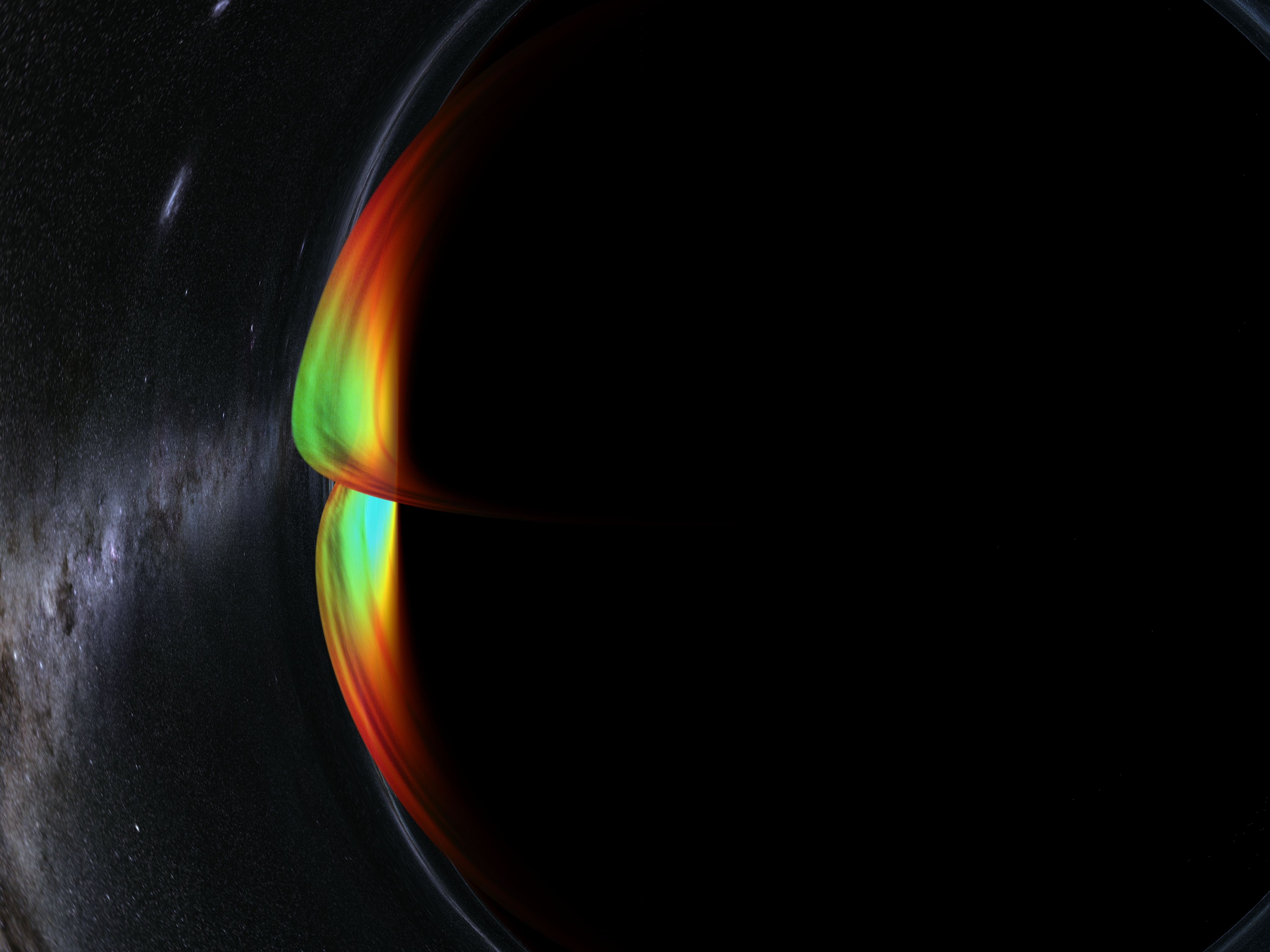
Note here that the side of the accretion disk that is pointing toward the observer shifts from the initial orange to yellow to green as the disk region approaches the gravitational center, increasing its circumferential velocity, but this reverses after a while and starts to turn yellow to red again as the gravitational redshift of proximity to the horizon overwhelms the Doppler blueshift from velocity.

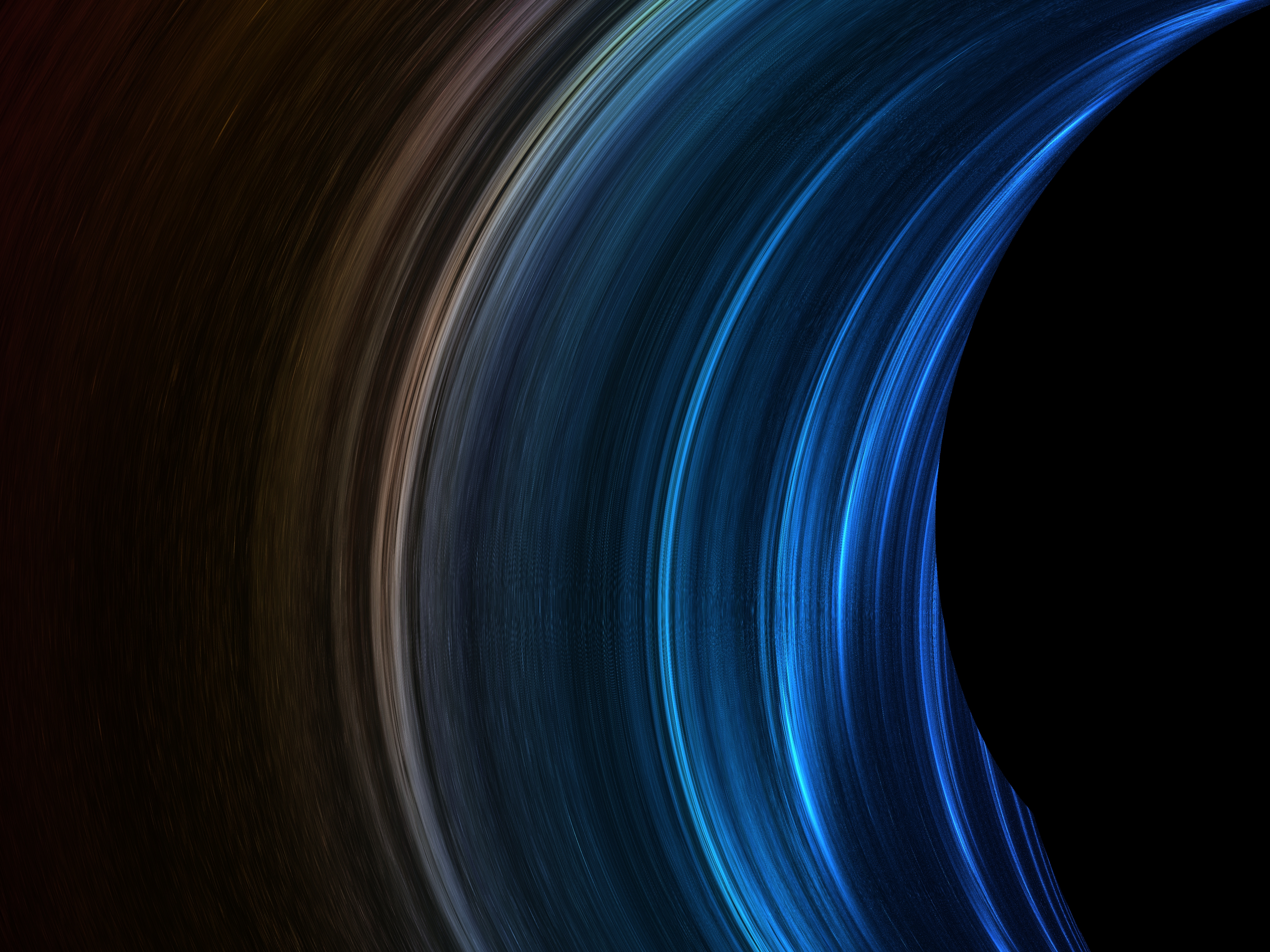
The second image is a close-up of a Kerr black hole with a spin of 0.999, where the bending from the rotation already changes the convexity at the equator.